Fundamental problems in Unsupervised Learning, such as Clustering and Dimensionality Reduction, can be fruitfully interpreted from the point of view of Topological Inference. This is an introduction to this point of view.

Topology
Topological Inference and Persistent Homology
Beyond Persistent Homology: Topological Inference in Unsupervised Learning
- Topology and Clustering
- Topology and Dimensionality Reduction

Topology

Topology is the branch of mathematics that studies the properties of spaces that remain unchanged under continuous deformations. For example, the number of connected components of a planar graph, such as $G_1$ below, is independent of how the graph is drawn: it does not depend, for example, on how long the edges are. Mathematicians say that the number of connected components is a topological invariant of the graph. On the other hand, the distance between a pair of vertices is not a topological invariant: it can change if the graph is drawn differently.

graphs

The number of connected components of a topological space $X$ is one of the simplest topological invariants, and it is called the zeroth Betti number of the space, and denoted $\beta_0(X)$. The first Betti number, denoted $\beta_1(X)$, counts the number of “one-dimensional holes”. For example, the space $S^1$ given by the circumference of a circle has a single one-dimensional hole $\beta_1(S^1) = 1$ and a single connected component $\beta_0(S^1) = 1$.

spaces

Holes come in all dimensions: for instance, a two-dimensional sphere $S^2$, such as a basketball, has a two-dimensional hole $\beta_2(S^2) = 1$ (its “inner void”), no one-dimensional holes $\beta_1(S^2)=0$, and a single connected component $\beta_0(S^2) = 1$. Another cool topological space is the surface of a donut (usually called a torus) denoted as $T$ in the picture above.

Topological spaces are continuous entities with potentially infinitely many points. A simplicial complex is a special kind of topological space that can be described using a finite amount of data. A simplicial complex is essentially an undirected hypergraph: like a graph, it can have vertices (called $0$-simplices) and edges (called $1$-simplices), but it can also have $n$-simplices for $n \geq 2$. For example, a $2$-simplex is a filled triangle, and a $3$-simplex is a filled tetrahedron. Here are the three spaces above represented as simplicial complexes:

simplicial-complexes

Topological Inference and Persistent Homology

Topological Inference is about estimating topological properties of spaces from incomplete information. A classical example is [Niyogi et al. DGC], which provides a statistically consistent algorithm for estimating the Betti numbers of a manifold from a finite sample. Topological Inference relates to the following keywords:

Computational Topology: the algorithmic computation of topological invariants.

Topological Data Analysis: theory and algorithms related to the usage of topological methods in data analysis, part of the broader fields of Geometric Data Science and Geometric Machine Learning.

Persistent Homology (PH): a particular construction with applications in Topological Inference and abstract Mathematics. Roughly speaking, PH provides a generalization of the concept of Betti number (sometimes called persistent Betti number or barcode) that applies to families of topological spaces, rather than to single topological spaces.

Here’s the typical toy example showcasing PH as a finite sample estimator for the Betti numbers of the circle $S^1$:

Persistent Homology has had several successes in the analysis of data coming from scientific applications. Cool examples include PH as a feature for the classification of cells in subcellular spatial transcriptomics^{[Benjamin et al. Nature]}, and PH as a means to detect and quantitatively describe center vortices in $SU(2)$ lattice gauge theory in a gauge-invariant way^{[Sale et al. Phys. Rev. D]}. More examples can be found at the DONUT database.

Beyond PH: Topology in Unsupervised Learning

Unsupervised Learning is the branch of Machine Learning concerned with unlabeled data, but exactly what this means will depend on whom you ask. For example, should self-supervision, as done in the pretraining phase of large language models, be regarded as Unsupervised Learning? For concreteness, let’s focus on a class of unsupervised learning techniques that is best represented by the following two classical problems:

The clustering problem: the problem of grouping data points of an unlabeled dataset into meaningful clusters.
The dimensionality reduction problem: the problem of representing an unlabeled dataset as a subset of a well-understood metric space, such as a Euclidean space, in a geometrically meaningful way.

The mathematical models underlying many of the approaches to these problems have a nice topological interpretation, as I now describe. I thank Leland McInnes for various conversations on these topics.

Topology and Clustering

Many clustering algorithms are in essence Topological Inference algorithms, designed to estimate the connected components of high-density regions of the sample distribution. This is done by estimating connectivity structure, typically with a graph, and then taking connected components.

A motivating example. As a starting point, let’s consider the most standard clustering algorithm: $k$-means. Informally, $k$-means assumes that the input data is sampled from a set of “blob-shaped” clusters, and seeks to assign each data point to its corresponding blob. More formally, the algorithm is an instance of the expectation-maximization procedure applied to a Gaussian mixture model with equal isotropic covariances, equal priors, and hard assignments. Mathematically, the model is the limit of the mixture $\frac{1}{k} \sum_{i=1}^k \mathcal{N}(\mu_i, \sigma^2\, \mathrm{I})$ as $\sigma^2 \to 0$. The model gives a precise mathematical meaning to the clusters that one seeks: these are represented by the means $\mu_i$, which correspond to the modes of the distribution. Thus, after estimating the means $\mu_i$, there is no need to estimate any connectivity structure directly, since points can be clustered by mapping them to their closest mode.

I like this interpretation of $k$-means because it naturally leads to density-based clustering, which can be roughly thought of as a non-parametric version of $k$-means.

Density-based clustering. In the simplest incarnation of density-based clustering, the data is assumed to be sampled from a distribution with probability density function $f : \mathbb{R}^n \to \mathbb{R}$, and the clusters are declared to be the “high-density regions” with respect to $f$. This can be made precise in a few ways. The simplest is to fix a threshold $\lambda \in \mathbb{R}$, and define the clusters at level $\lambda$ to be the connected components of the $\lambda$-superlevel set $\{x \in \mathbb{R}^n : f(x) \geq \lambda\}$, like so:

density-based-clustering

A standard density-based clustering algorithm based on this principle is DBSCAN ^{[Ester et al. KDD]}, which, as observed¹ in [McInnes, Healy. ICDMW], can be recast as the combination of two main tools:

A kernel density estimator, from Statistics.
A Rips complex, from Topological Inference.

The Rips complex at scale $\varepsilon$ has as vertices the data points, and puts an edge between each pair of data points at distance at most $\varepsilon$. The Rips complex already showed up earlier in the figure illustrating PH. Here’s the Rips complex of a tiny point cloud at a fixed scale $\varepsilon$:

rips

DBSCAN has two parameters, often denoted $\varepsilon$ and $k$. The parameter $k$ plays the role of the threshold $\lambda$, above. The parameter $\varepsilon$ is more interesting, and has two uses: as the width parameter for the kernel density estimator, and as the scale parameter for the Rips complex. So $\varepsilon$ is used for both Statistical Inference (density properties of the data) and Topological Inference (connectivity properties of the data).

Hierarchical clustering. If one does not want to, or does not know how to choose the threshold $\lambda$, one enters the realm of hierarchical clustering. Going back to the probability density function $f : \mathbb{R}^n \to \mathbb{R}$, if one lets $\lambda$ vary from larger to smaller, the superlevel sets of $f$ are nested, meaning that the $\lambda_1$-superlevel set is included in the $\lambda_2$-superlevel set whenever $\lambda_1 \geq \lambda_2$. By considering the connected components of all the superlevel sets, one obtains a hierarchical clustering, sometimes known as a cluster tree, which keeps track of how the connected components of the superlevel sets of $f$ appear and merge. The cluster tree can be summarized using PH, allowing one to quantify the prominence of modes and high density regions, and to do cluster inference robustly.

cluster-tree

Similarly, one can fix one of the two parameters of DBSCAN and let the other one vary, to obtain a hierarchical clustering algorithm that consistently estimates the cluster tree^{[Chaudhuri, Dasgupta. NeurIPS][Chazal et al. JACM]}. This is, in essence, a version of the HDBSCAN algorithm, in case you have heard of it.

Even more, one can let both parameters of DBSCAN vary and obtain a two-parameter hierarchical clustering algorithm, which is also consistent and contains many standard hierarchical clusterings as “one-dimensional slices”. This is introduced in [Rolle, Scoccola. JMLR] and is implemented in our Python package persistable-clustering. It makes use of a density-sensitive generalization of the Rips complex from Topological Inference, called degree-Rips.

degree-rips

Topology and Dimensionality Reduction

Many non-linear dimensionality reduction algorithms also start with a Topological Inference phase, where a graph or simplicial complex is constructed, which is then used as a proxy for the space the data is assumed to be sampled from.

A motivating example. A classical example is Laplacian Eigenmaps (LE)^{[Belkin, Niyogi. Neural Comput.]}, which starts by constructing a graph estimating the connectivity of the data. This graph is then weighted using distance information, since the next step is to use it as a proxy for a manifold to estimate the Laplacian eigenfunctions, which are then used to find a low-dimensional embedding. The weighing is strictly speaking Geometric Inference, since its goal is to estimate geometric properties. It is only natural that Topological and Geometric Inference often show up together.

Uniform Manifold Approximation and Projection (UMAP). A more modern non-linear dimensionality reduction algorithm is UMAP^{[McInnes et al.]}, which has become the go-to algorithm for lots of applications. UMAP shares many similarities with LE, and in fact relies on LE for initialization, but the theoretical justification for UMAP is more topological in nature, and uses weighted simplicial complexes in a crucial way. In essence, the data is modelled as a probabilistic simplicial complex for which a low-dimensional embedding is found using stochastic gradient descent and clever computational shortcuts. I am skipping over lots of interesting details here; besides the original paper, I recommend the documentation for the official implementation, and other online resources, such as the interactive blogpost [Coenen, Pearce], from where I took the following illustrative example:

coenen-pearce

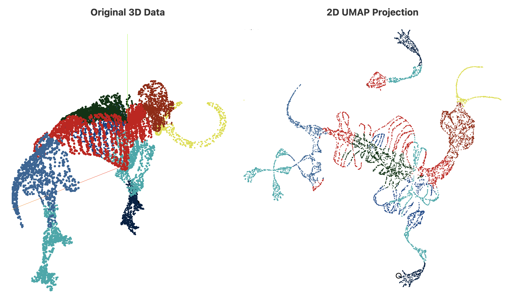
In practice, UMAP is robust to many kinds of noise and data imperfections, and it is an excellent starting point in many scenarios, including exploratory data analysis. However, as opposed to the clustering techniques that I described earlier, it does not come with theoretical guarantees (at least for the moment), and interpretability may not be straightforward.

Next, I’ll describe a topological dimensionality reduction procedure that is limited in scope and less robust, but that, thanks to this, admits theoretical guarantees and higher interpretability.

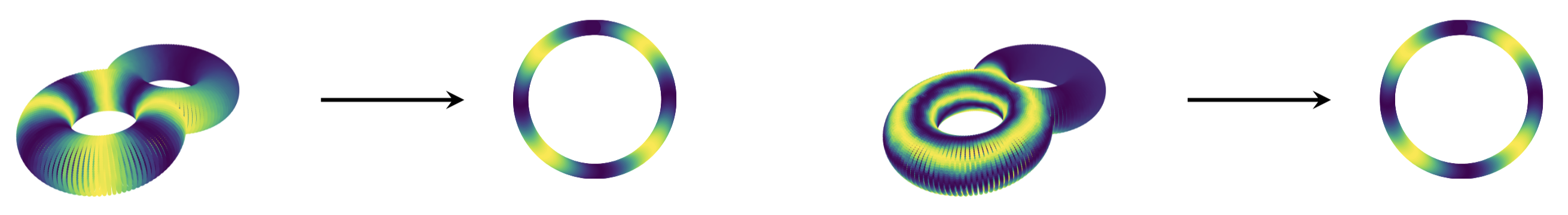
The circular coordinates algorithm. The motivating question is the following: Given a space $X$ with a one-dimensional hole, does there exist a function $f : X \to S^1$ from the space to the circle that parametrizes this hole?

Such function $f$ would provide us with a topologically faithful representation of $X$, at least when it comes to preserving its circularity. For example, here are two functions from a “double-torus” to the circle, which parametrize two of its one-dimensional holes:

circular-coordinates

A standard theorem from topology (sometimes called the representability theorem for cohomology) guarantees that such function $f$ always exists; moreover, if $X$ is a Riemannian manifold, then there is a canonical choice for such function: the one with minimal Dirichlet energy. The exact meaning of this is not crucial; what matters is that, given a finite sample of a space with a one-dimensional hole, a bit of Topological and Geometric Inference gives us back a map from the sample to the circle $S^1$. This procedure is known as the circular coordinates algorithm^{[de Silva, Vejdemo-Johansson. SoCG]}, and is implemented in our Python package DREiMac, which was used, for instance, in Neuroscience^{[Schneider et al. Nature]}. Another interesting source of circularity in data is periodicity and quasiperiodicity in time series^{[Perea et al. BMC Bioinformatics]}.

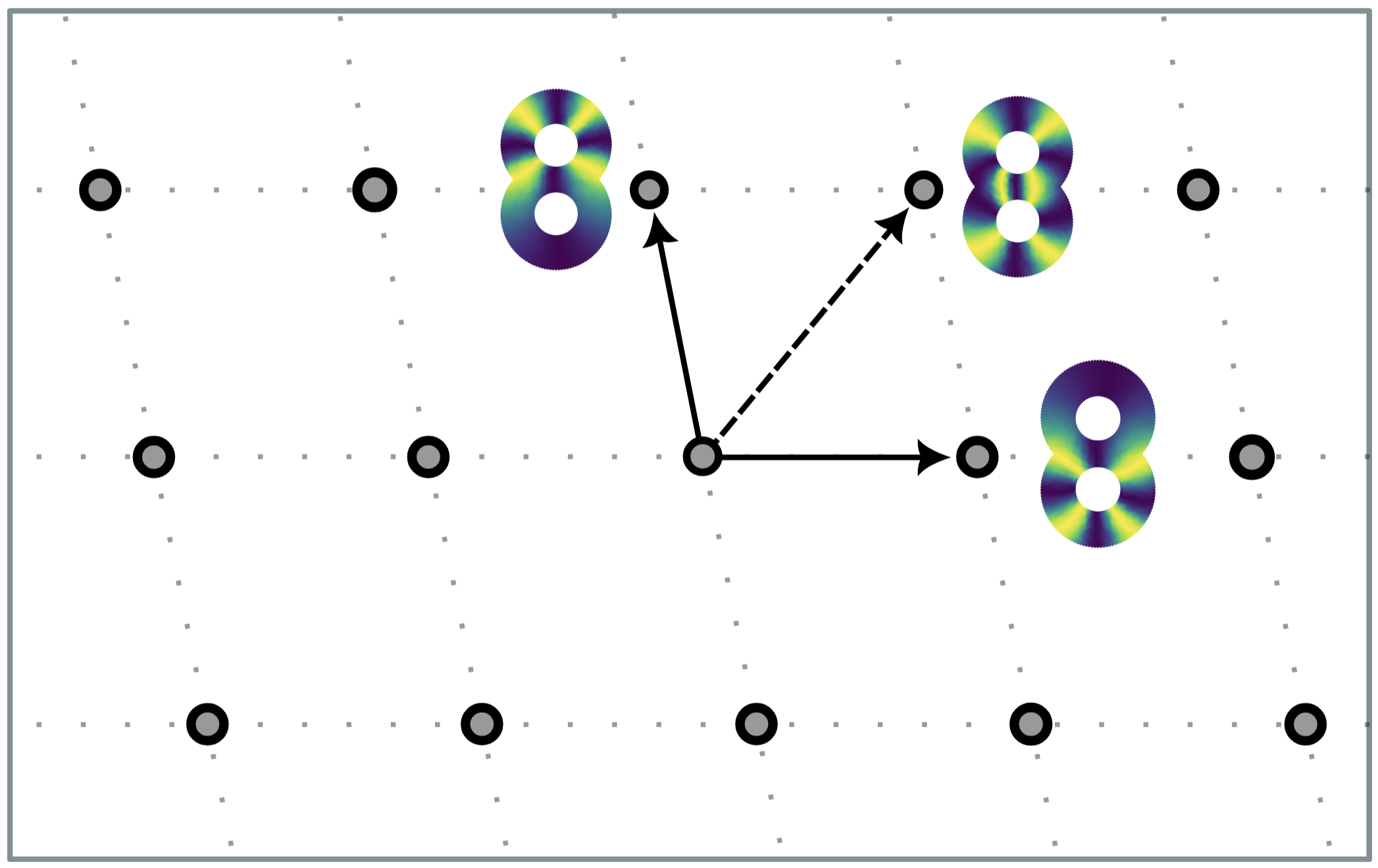
The toroidal coordinates algorithm. There exists examples where data can have more than one one-dimensional hole. For instance, [Gardner et al. Nature] shows that the population activity of grid cells (part of the neural system concerned with an individual’s position) resides on a topological torus. When dealing with a sample from a space $X$ with more than one one-dimensional hole $\beta_1(X) = n \geq 2$ the original circular coordinates algorithm often outputs circle-valued maps that are “geometrically correlated”, and which are thus harder to interpret. In [Scoccola et al. SoCG], we make formal the notion of geometric correlation for circle-valued maps using the Dirichlet form, which endows the set of circle-valued maps with the structure of a lattice:

dirichlet-form

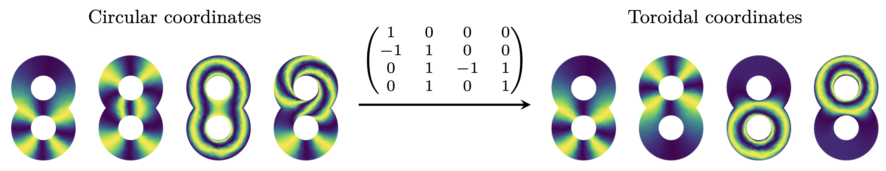
In that paper, we describe the toroidal coordinates algorithm, which enhances the circular coordinates algorithm by “decorrelating” the circle-valued maps. Informally, this decorrelation is an analogue of PCA for maps into a product of circles (rather than maps into a product of real lines). The difficulty is that a product of circles is not a vector space, so the projection matrix is constrained to have integer entries. We addressed this using lattice reduction, a method from Computational Number Theory:

lattice-reduction

The toroidal coordinates algorithm is also implemented in DREiMac. There also exist other topological dimensionality reduction algorithms, which parametrize topological features other than circularity, such as the one in [Schonsheck, Schonsheck. JACT].

What’s next? In the world of Dimensionality Reduction, the gap between theoretical guarantees and practical methods is much wider than in Clustering, where, as described earlier, there exist practical methods with strong topology recovery guarantees. Non-linear dimensionality reduction methods with theoretical guarantees have limited scope and tend not to be very robust, while general purpose methods that are efficient and robust tend to be justified by heuristics. This is not surprising: Dimensionality Reduction is more complicated than clustering, and higher dimensional topological invariants are more complicated than the connected components.

Perhaps the practical Dimensionality Reduction method with the strongest available guarantees is Laplacian Eigenmaps, for which geometric consistency has been established a while ago^{[Belkin, Niyogi. NeurIPS]}. But, to the best of my knowledge, the topological properties of the LE embedding are not well understood beyond connected components.

What would be really nice to see is any of the following:

Methods that lie in-between UMAP and the topological parametrization methods, and which enjoy the good properties of both. This could be, for example, making UMAP more interpretable or making the topological parametrization methods more widely applicable and robust.
Theoretical guarantees for at least some parts of the UMAP pipeline or a suitably modified pipeline.
In particular, I would like to see topological consistency results for the nearest neighbor graph construction. While a lot is known about the Rips complex, it’s sibling, the nearest neighbor graph (ubiquitous in non-linear dimensionality reduction methods) has been mostly neglected when it comes to Topological Inference. The only related paper that I can remember is [Berry, Sauer. FoDS], which establishes geometric consistency.

If you know of interesting work in these directions, feel free to contact me!

To be fully precise, it is the algorithm DBSCAN* that exactly has that form. DBSCAN* is a minor modification of DBSCAN introduced in [Campello et al. KDD]. ↩